Feedback

Feedback is an amazingly useful tool in electronics. When negative, it allows us to use the gain of an amplifier as a currency that we can spend to get more bandwidth, less noise, improve input-output impedances, and many other things. Positive feedback is also quite useful: we make oscillators and hysteresis comparators with it.

Generally we look at a circuit and figure out which feedback type is being applied to it (positive or negative) by analysing the feedback loop, and that’s it. Now, consider the following circuit:

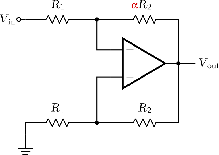
In this case, there are two feedback loops in paralel. One positive and one negative, and one of them will dominate depending on the value of $\alpha$. To analyse this, we can completely disregard the input source, shorting it to ground.

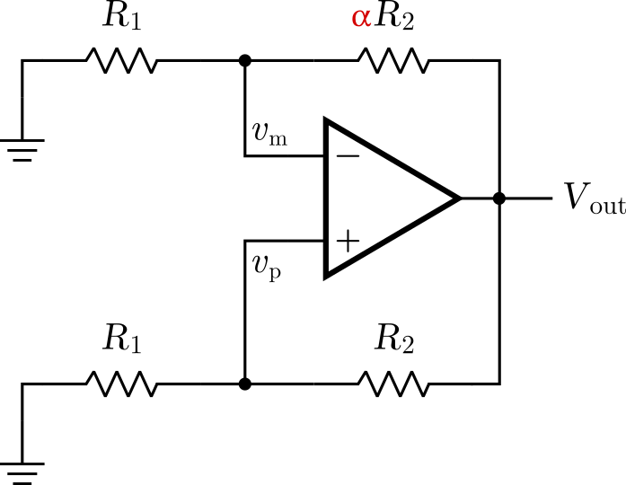
Now, if more of the output goes to the negative input $v_m$ than to the positive $v_p$, the feedback will be overall negative. So, to have negative feedback, we should ensure that

Conversely, feedback will be positive if $\alpha>1$, but what happens when $\alpha=1$? Well, in this case the positive and negative feedbacks will cancel out and the amplifier will behave more or less like its open-loop version.

Here is a fun animation of what happens when sweeping $\alpha$ from $0$ to $2$. We can see it changing from an inverter amplifier to a hysteresis comparator, all as a result of changing one resistance!

Intuitive conclusions

In this example we saw how the value of a passive component on a circuit can make it change feedback types from negative (usually desired) to positive (usually undesired). Therefore, be very careful about variability in your supposedly stable circuits!

If you ignore this possibility, unavoidable device variations can put you in a tricky situation at a point in time when you cannot change the circuit anymore.

To back up the intuitive analysis that I presented here, I brought a more in-depth circuit analysis that can be used to find the circuit behavior for every value of $\alpha$.

In-depth analysis

To derive a general expression for this circuit, we cannot assume anything about the feedback. Considering that the circuit acts instantaneously, we can write its output for a given time $t+\delta$, such that $\delta$ is infinitesimal, as

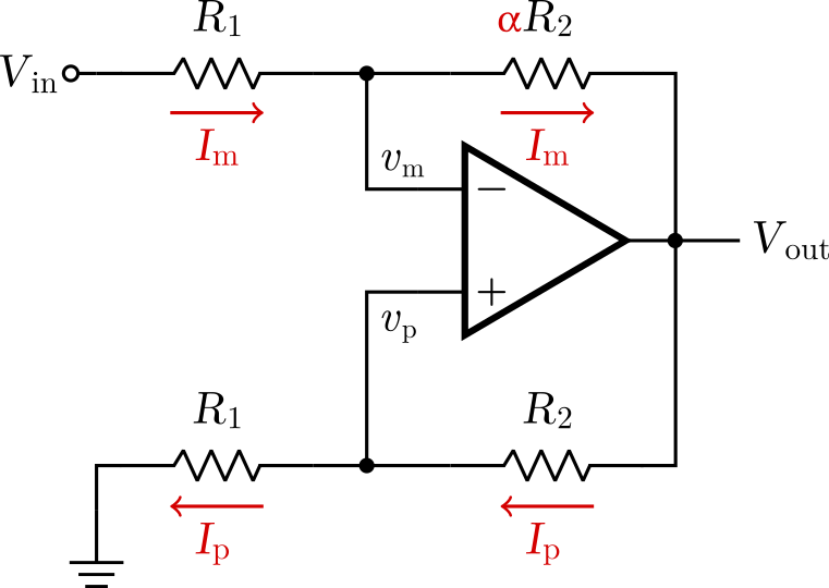
In this case, $v_p$ and $v_m$ can also depend on $V_{in}$ as a function of the resistances. As the following figure shows, the current $I_m$ is the same across all the top branch, while $I_p$ is constant across the bottom branch.

Thus, we can deduce that

Bringing those values together to the first expression gives

From (8) it we can derive the circuit behavior for any value of $\alpha$. Note how the term being multiplied by $V_{out}$ is the same I used before in the quick analysis to determine the feedback type. Now we can see in the output equation itself that if the term is positive (or negative), the output will be fed back positively (or negatively) to the evaluation of the next output.

Let’s now see what happens in each case.

Case 1: setting $\alpha = 1$

In this situation,

setting the first term of (8) to zero, therefore

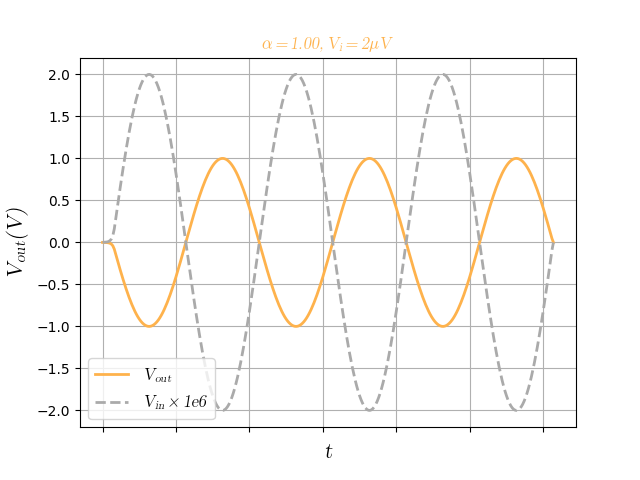
That’s what I meant when I said earlier that the circuit would behave more or less like its open-loop version. It actually has negative gain, and it will be reduced by a factor of a voltage divider.

Giving it some values, I considered $A = 1MV/V$, $R_1 = R_2 = 10k\Omega$, and $V_{in}$ as a sinusoid with $2\mu V$ amplitude. This case will lead to a final gain of $500k$. Here is the output:

Case 2: setting $\alpha = 0.5$

In this case, the feedback is negative and the system is stable. Thus, $V_{out}(t+\delta) = V_{out}(t)$ for any given time, being a function of only $V_{in}$. After some rearranging, taking this into account in (8) leads to,

If we assume $A$ to be sufficiently big, it leads to

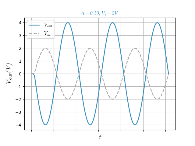
This is a quite funny expression. It reminds us of the gain equation for the non-inverting amplifier, but in this case it is also inverting. Also, there is a quite elegant dependance on $\alpha$.

To give it some values, let’s consider $A = 1MV/V$, $R_1 = R_2 = 10k\Omega$, and $V_{in}$ as a sinusoid with $2 V$ amplitude. This case will lead to a final gain of $2$. Here is the output:

Case 3: setting $\alpha = 2$

In this case, the positive feedback would render this system unstable. However, since op-amps saturate their output voltage on $\pm VDD$ (ideally), the system becomes nonlinear, with two stable equilibrium points, showing hysteretic behavior.

The analysis here also refers back to equation (8). I’m rewriting it for readability:

Since the gain $A$ is quite big, if the right-hand side of this equation is positive, the op-amp will saturate to $VDD$. If it is negative, the output at ($t+\delta$) will be $-VDD$. To make the RHS positive, it means that

After some manipulation, this inequality becomes

Reverting the inequality, we obtain that

At $\alpha=2$, $R_1 = R_2 = 10k \Omega$, and $VDD=5V$, the hysteresis curve transitions at $\pm 1.25V$. Here is the output of a time-simulation using a sinusoid of 2V amplitude:

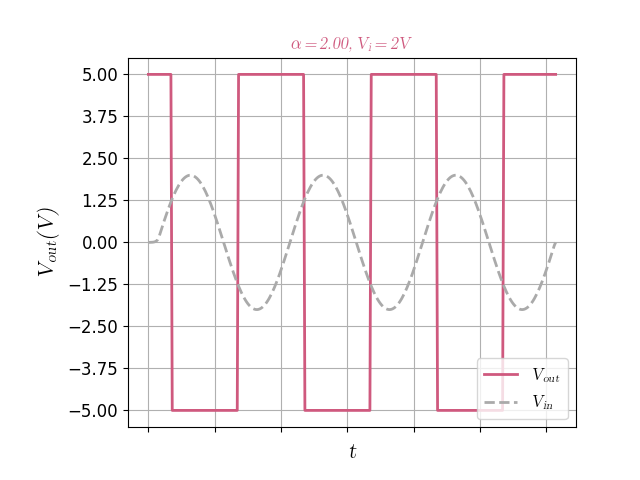
In the figure we can see that, once the sinusoid hits over $1.25V$, the output goes to $-VDD$ and stays at it, even when the input is lower than the $1.25V$. It only transitions again once $V_{in}$ is as low as $-1.25V$, which proves it has hysteresis.

Conclusions

It is very interesting how elegant and full of insight such a simple circuit can be. Hopefully now you see the beauty of its behavior as I do. Here is the transfer characteristic animation once again.

I would like to finish with a special thanks to professor Hamilton Klimach, who showed me this topology and strongly suggested me to simulate it!

That’s it for me today. Thanks for reading and I wish you have a great day!